Deep Learning Using TensorFlow
Summary
The purpose of this exercise is to use deep neural networks to classify traffic signs. Specifically, we train a model to classify traffic signs from the German Traffic Sign Dataset.
Data
The pickled data is a dictionary with 4 key/value pairs:
- features -> the images pixel values (width, height, channels)
- labels -> the label of the traffic sign
- sizes -> the original width and height of the image (width, height)
- coords -> coordinates of a bounding box around the sign in the image, (x1, y1, x2, y2). Based the original image (not the resized version).
# Hide warnings
import warnings
warnings.filterwarnings('ignore',category=DeprecationWarning)

# Load required libraries
import pickle
import numpy as np
import cv2
import tensorflow as tf
import matplotlib.pyplot as plt
from sklearn.preprocessing import LabelBinarizer
from sklearn.cross_validation import train_test_split
from tqdm import tqdm
from scipy import misc
import os
import pandas as pd
# Load pickled data

# Open training and testing data files
training_file = 'data/train.p'
testing_file = 'data/test.p'

with open(training_file, mode='rb') as f:
    train = pickle.load(f)
with open(testing_file, mode='rb') as f:
    test = pickle.load(f)

X_train, y_train = train['features'], train['labels']
X_test, y_test = test['features'], test['labels']
Data Exploration
Basic Data Summary
# Number of training examples
n_train = len(X_train)

# Number of testing examples
n_test = len(X_test)

# The shape of an image
image_shape = X_train.shape[1:]

# Number of classes in the dataset
n_classes = len(np.unique(y_train))

print("Number of training examples =", n_train)
print("Number of testing examples =", n_test)
print("Image data shape =", image_shape)
print("Number of classes =", n_classes)
Number of training examples = 39209
Number of testing examples = 12630
Image data shape = (32, 32, 3)
Number of classes = 43
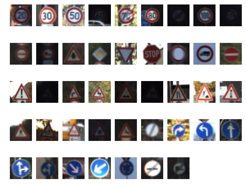
Pictures of the signs
traffic_sign = []

for i in range(0,n_classes):
    plt.subplot(5,9,i+1)
    traffic_sign.append(X_test[np.where( y_test == i )[0][0],:,:,:].squeeze())
    img = plt.imshow(X_test[np.where(y_test == i)[0][0],:,:,:].squeeze())
    plt.axis('off')
 /images
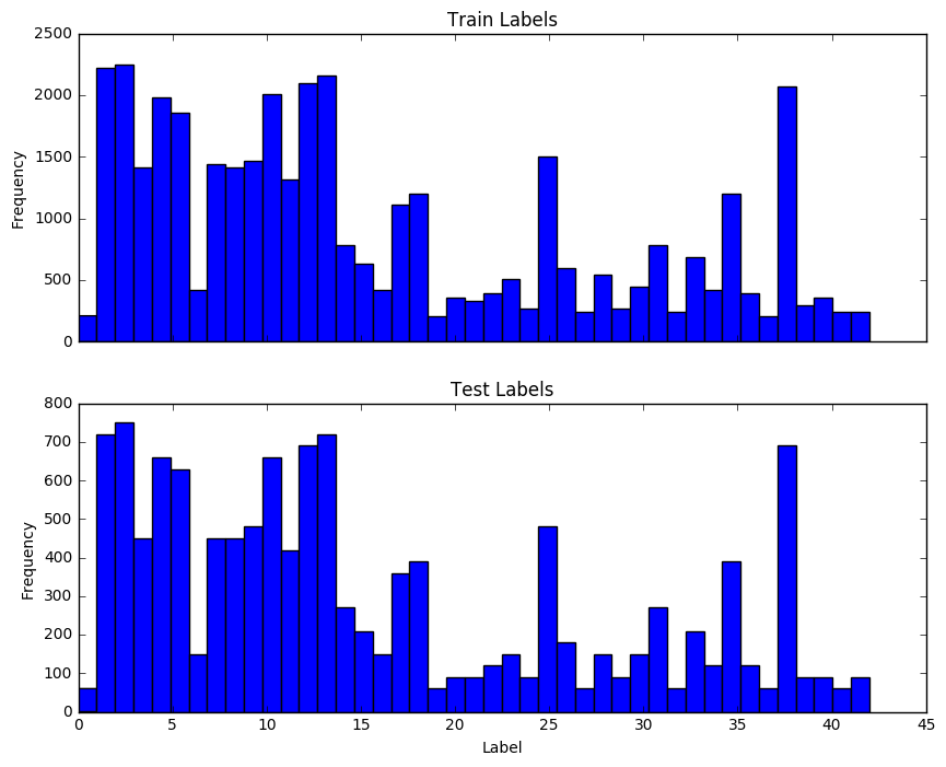
Count of each sign
# Plot histogram of labels in training and test set
f, axarr = plt.subplots(2, sharex = True)
axarr[0].hist(y_train, bins = n_classes)
axarr[0].set_title('Train Labels')
axarr[0].set_ylabel('Frequency')
axarr[1].hist(y_test, bins = n_classes)
axarr[1].set_title('Test Labels')
axarr[1].set_xlabel('Label')
axarr[1].set_ylabel('Frequency')
<matplotlib.text.Text at 0x12ab24be0>
Data Preprocessing
Whenever possible, we want our variables to have 0 mean and equal variance when performing gradient descent optimization. One way we can do this on images is to convert the images to greyscale. This has the effect of reducing the overall variation in the dataset. However, we would like to preserve the variation between colors so the normalization was performed individually on each color.
Also, in order to convert labels into numbers, I applied One-Hot Encoding.
Implement Min-Max scaling to convert image to greyscale
# Implement Min-Max scaling for greyscale image data
def normalize_greyscale(image_data):
    """
    Normalize the image data with Min-Max scaling to a range of [0.1, 0.9]
    :param image_data: The image data to be normalized
    :return: Normalized image data
    """
    # ToDo: Implement Min-Max scaling for greyscale image data
    a = 0.1
    b = 0.9
    greyscale_min = 0
    greyscale_max = 255
    return a + (((image_data - greyscale_min)*(b - a))/(greyscale_max - greyscale_min))

X_test_n = numpy.zeros((X_test.shape[0], X_test.shape[1]*X_test.shape[2], X_test.shape[3]), dtype=float)
X_train_n = numpy.zeros((X_train.shape[0], X_train.shape[1]*X_train.shape[2], X_train.shape[3]), dtype=float)

for i in range (X_test.shape[3]):
    X_test_n[:,:,i] = normalize_greyscale(X_test[:,:,:,i].reshape(X_test.shape[0], X_test.shape[1]*X_test.shape[2]))
    X_train_n[:,:,i] = normalize_greyscale(X_train[:,:,:,i].reshape(X_train.shape[0], X_train.shape[1]*X_train.shape[2]))

X_test_n = X_test_n.reshape(X_test_n.shape[0], X_test_n.shape[1]*X_test_n.shape[2])
X_train_n = X_train_n.reshape(X_train_n.shape[0], X_train_n.shape[1]*X_train_n.shape[2])
Apply One-Hot Encoding
# Turn labels into numbers and apply One-Hot Encoding
encoder = LabelBinarizer()
encoder.fit(y_train)
y_train = encoder.transform(y_train)
y_test = encoder.transform(y_test)

# Convert to float32
y_train = y_train.astype(np.float32)
y_test = y_test.astype(np.float32)
Split the data into training/validation sets
The train_test_split function was used to separate the data in training and validation sets (70/30 split)
# Get randomized datasets for training and validation
train_features, valid_features, train_labels, valid_labels = train_test_split(
    X_train_n,
    y_train,
    test_size=0.3,
    random_state=832289)
Model Architecture
The model used in this classification task is the Feedforward Neural Network. It contains 2 hidden layers. Within each layer, ReLU is used to convert the linear models into non-linear models. The cost function is determined using the softmax_cross_entropy_with_logits method.
The size of each layer was 3072.
After testing several methods for the optimizer, I settled on using the AdamOptimizer method for the optimizer since it produced the most accurate results. I used a learning rate of 0.001, 20 training epochs and a batch size of 1000.
The accuracy against the test set is determined to be 0.76.
# Learning Parameters
learning_rate = 0.001
training_epochs = 20
batch_size = 1000

# Size of inputs
n_input = train_features.shape[1]
n_classes = train_labels.shape[1]

# Hidden Layer Parameters
n_hidden_layer1 = n_input # layer 1: number of features
n_hidden_layer2 = n_input # layer 2: number of features

# Store layers weight & bias
weights = {
    'hidden_layer1': tf.Variable(tf.random_normal([n_input, n_hidden_layer1], mean = 0, stddev = 0.01)),
    'hidden_layer2': tf.Variable(tf.random_normal([n_hidden_layer1, n_hidden_layer2], mean = 0, stddev = 0.01)),
    'out': tf.Variable(tf.random_normal([n_hidden_layer2, n_classes]))
}
biases = {
    'hidden_layer1': tf.Variable(tf.random_normal([n_hidden_layer1], mean = 0, stddev = 0.01)),
    'hidden_layer2': tf.Variable(tf.random_normal([n_hidden_layer2], mean = 0, stddev = 0.01)),
    'out': tf.Variable(tf.random_normal([n_classes]))
}

# tf Graph input
x = tf.placeholder("float", [None, n_input])
y = tf.placeholder("float", [None, n_classes])

# Hidden layers with RELU activation
layer_1 = tf.add(tf.matmul(x, weights['hidden_layer1']), biases['hidden_layer1'])
layer_1 = tf.nn.relu(layer_1)

layer_2 = tf.add(tf.matmul(x, weights['hidden_layer2']), biases['hidden_layer2'])
layer_2 = tf.nn.relu(layer_2)

# Output layer with linear activation
logits = tf.matmul(layer_2, weights['out']) + biases['out']

prediction = tf.nn.softmax(logits)
predict = tf.argmax(logits, 1)

# Define loss and optimizer
loss = tf.reduce_mean(tf.nn.softmax_cross_entropy_with_logits(logits, y))
optimizer = tf.train.AdamOptimizer(learning_rate=learning_rate).minimize(loss)

# Define accuracy
is_correct_prediction = tf.equal(tf.argmax(prediction, 1), tf.argmax(y, 1))
accuracy = tf.reduce_mean(tf.cast(is_correct_prediction, tf.float32))

# Initialize storage variables
loss_batch = []
train_acc_batch = []
valid_acc_batch = []

# Initialize tf session
sess = tf.Session()
sess.run(tf.initialize_all_variables())

# Run for all epochs
for epoch in range(training_epochs):

    # The training cycle
    for batch_start in range(0, train_labels.shape[0], batch_size):
        batch_finish = batch_start + batch_size
        batch_features = train_features[batch_start:batch_finish]
        batch_labels = train_labels[batch_start:batch_finish]

        # Run optimizer
        sess.run(optimizer, feed_dict = {x: batch_features, y: batch_labels})

    loss_out = sess.run(loss, feed_dict={x: batch_features, y: batch_labels})
    acc = sess.run(accuracy, feed_dict = {x: batch_features, y: batch_labels})
    loss_batch.append([loss_out])
    train_acc_batch.append([acc])

    acc = sess.run(accuracy, feed_dict = {x: valid_features, y:  valid_labels})
    valid_acc_batch.append([acc])

# Check accuracy against Validation data
test_accuracy = sess.run(accuracy, feed_dict = {x: X_test_n, y:  y_test})

# Plot Loss and Accuracy
epochs = np.arange(training_epochs)
loss_plot = plt.subplot(211)
loss_plot.set_title('Loss')
loss_plot.plot(epochs, loss_batch, 'r')
loss_plot.set_xlim([epochs[0], epochs[-1]])
acc_plot = plt.subplot(212)
acc_plot.set_title('Accuracy')
acc_plot.plot(epochs, train_acc_batch, 'g', label='Training Accuracy')
acc_plot.plot(epochs, valid_acc_batch, 'b', label='Validation Accuracy')
acc_plot.set_ylim([0, 1.0])
acc_plot.set_xlim([epochs[0], epochs[-1]])
acc_plot.legend(loc=4)
plt.tight_layout()
plt.show()

print('Test set accuracy at {}'.format(test_accuracy))
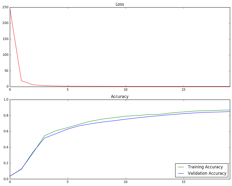
Test set accuracy at 0.7630245685577393
Test a Model on New Images
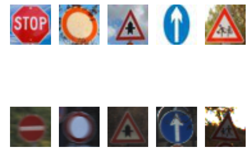
5 random images were selected from the web and the above model was used to classify each image
# Load the data
signs = []
for filename in os.listdir('signs'):
    sign = plt.imread('signs/' + filename)
    signs.append(sign)

# Plot the signs
fig = plt.figure()
fig.add_subplot(2,3,1)
plt.axis('off')
plt.imshow(signs[0])
fig.add_subplot(2,3,2)
plt.axis('off')
plt.imshow(signs[1])
fig.add_subplot(2,3,3)
plt.axis('off')
plt.imshow(signs[2])
fig.add_subplot(2,3,4)
plt.axis('off')
plt.imshow(signs[3])
fig.add_subplot(2,3,5)
plt.axis('off')
plt.imshow(signs[4])
plt.axis('off')
(-0.5, 31.5, 31.5, -0.5)
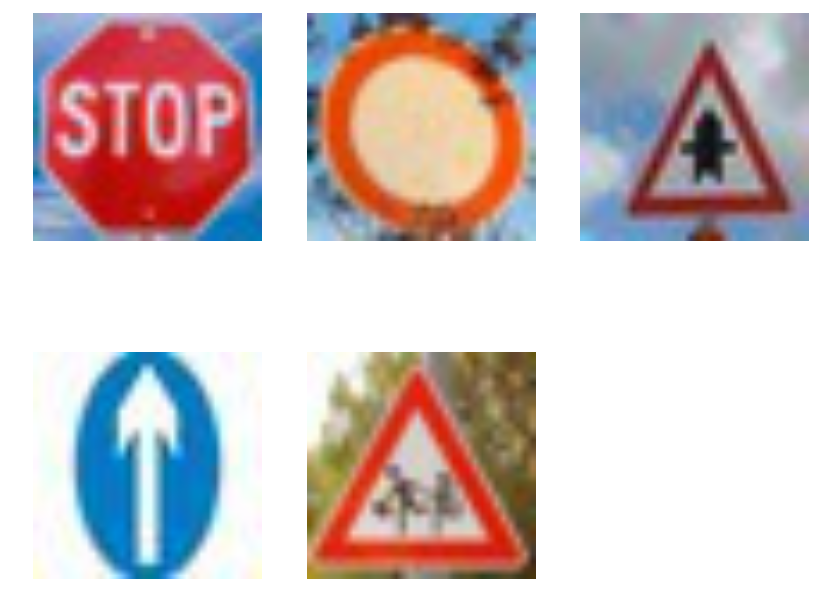
The second sign has a lot of obstruction to it with tree branches covering parts of the sign, in addition to containing different colors than those in the training set. I suspect that this one will be difficult to classify by the algorithm. There is also a slight tilt in a couple of the signs, thereby causing classification issues. Also, at this resolution and size, the images look quite blurred.
# Preprocess the images and run the signs through the prediction algorithm to test performance
X = np.array(signs)
X_mine = numpy.zeros((X.shape[0],X.shape[1]*X.shape[2],X.shape[3]), dtype=float)

for i in range (X.shape[3]):
    X_mine[:,:,i] = normalize_greyscale(X[:,:,:,i].reshape(X.shape[0], X.shape[1]*X.shape[2]))

X_mine = X_mine.reshape(X_mine.shape[0], X_mine.shape[1]*X_mine.shape[2])

preds = sess.run(predict, feed_dict = {x: X_mine})
print(preds)

fig = plt.figure()
for i in [1,2,3,4,5]:
    fig.add_subplot(2,5,i)
    plt.imshow(X[i-1,:,:,:])
    plt.axis('off')
    fig.add_subplot(2,5,i+5)
    plt.imshow(traffic_sign[preds[i-1]])
    plt.axis('off')
[17 15 11 35 28]
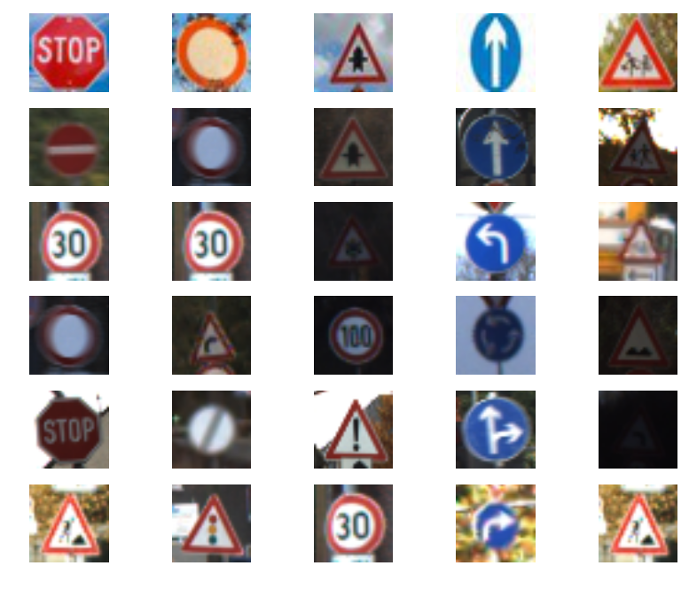
The model was able to predict 2 correctly out of 5. This accuracy level is considerably less than the test dataset. However, with a little more tuning, I believe that the accuracy can be considerably improved. The incorrect classifications are actually quite similar the correct image in most cases.
# Get top k performers
top_k = sess.run(tf.nn.top_k(prediction , k=5), feed_dict={x: X_mine})

top_k_t = pd.DataFrame(top_k.values.transpose())
top_k_t.plot(kind='bar').set_ylabel('Probability')

print(top_k.values)
print(top_k.indices)

fig = plt.figure()
for i in [1,2,3,4,5]:
    fig.add_subplot(6,5,i)
    plt.imshow(X[i-1,:,:,:])
    plt.axis('off')
    for j in [0,1,2,3,4]:
      fig.add_subplot(6,5,i+(j+1)*5)
      plt.imshow(traffic_sign[top_k.indices[i-1][j]])
      plt.axis('off')
[[  9.14724290e-01   3.48184742e-02   2.44188774e-02   1.12548526e-02
    8.70645326e-03]
 [  6.19467914e-01   1.66500613e-01   1.06849402e-01   3.82951796e-02
    1.47809843e-02]
 [  9.37286496e-01   4.40914296e-02   6.60394179e-03   4.35731094e-03
    2.27867719e-03]
 [  9.99963284e-01   2.19555932e-05   1.33507947e-05   1.26138286e-06
    1.20478603e-07]
 [  7.13300705e-01   1.70367077e-01   9.27464738e-02   2.05706917e-02
    1.45089917e-03]]
[[17  1 15 14 25]
 [15  1 20 32 26]
 [11 30  7 18  1]
 [35 34 40 36 33]
 [28 29 22 19 25]]
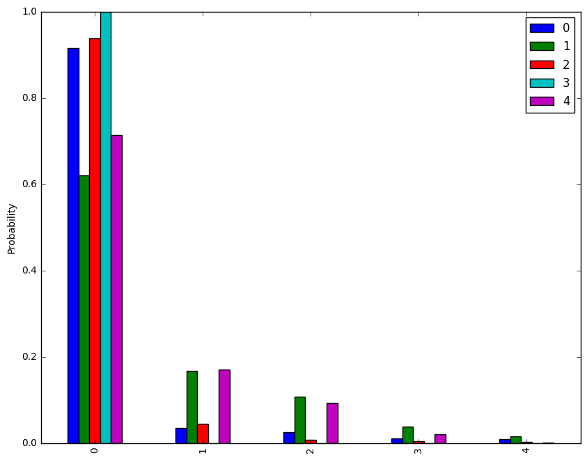
The model is fairly certain about the "Right-of-way at next intersection" and "Ahead only" signs with probabilities above 90%. The model was fairly certain about the "Student Crossing" sign. There was quite a bit of uncertainty about the other 2 signs. For the "No Vehicles" sign, the model gave the incorrect output. The correct output did not even appear in the top 5. As noted about, this was expected since the colors did not match the training dataset.