Purpose
The goal of this project is to identify employees from Enron that have been in on the fraud committed that came to light in 2001. This will be based on a machine learning algorithm using public Enron financial and email information.
Data Exploration
The dataset that will be used in this investigation to identify employees that may have committed fraud within Enron will be publicly available financial information. By breaking up the dataset into training and test sets and using our set of known POIs (Person Of Interest), we can use the features associated with each employee to identify whether or not they may be part of the fraud. This dataset contains a total of 146 points. Out of the 146 observations, 18 (12.3%) are POIs and 128 (87.7%) are therefore non-POIs. Each of the observations contains 21 features. Since this is a real-world dataset, not all of the features have attached values to them, hence showing up as NaNs. The list below provides the top 5 features the most missing values: 1. loan_advances: 142 NaNs 2. director_fees: 129 NaNs 3. restricted_stock_deferred: 128 NaNs 4. deferral_payments: 107 NaNs 5. deferred_income: 97 NaNs
#Import libraries
import warnings
warnings.filterwarnings('ignore', category=DeprecationWarning)
import sys
import pickle
sys.path.append("./tools/")
from feature_format import featureFormat, targetFeatureSplit
from tester import dump_classifier_and_data
import matplotlib.pyplot as plt
from sklearn.feature_selection import SelectKBest
import numpy as np
from sklearn.pipeline import Pipeline
from sklearn.preprocessing import MinMaxScaler
from sklearn.preprocessing import StandardScaler
from sklearn import tree
from sklearn.metrics import accuracy_score
from sklearn.grid_search import GridSearchCV
from sklearn.cross_validation import StratifiedShuffleSplit
from sklearn.decomposition import PCA
from sklearn.naive_bayes import GaussianNB
from sklearn.cross_validation import train_test_split
from sklearn import svm
from sklearn.svm import SVC
from sklearn import metrics
from sklearn import cross_validation
from tester import test_classifier

### Features List
### The first feature must be "poi".
### This features list contains all the features in the
### dataset (except email_address)

features_list = ['poi','salary', 'deferral_payments',
                    'total_payments', 'loan_advances',
                    'bonus', 'restricted_stock_deferred',
                    'deferred_income', 'total_stock_value',
                    'expenses', 'exercised_stock_options',
                    'other', 'long_term_incentive', 'restricted_stock',
                    'director_fees','to_messages',
                    'from_poi_to_this_person', 'from_messages',
                    'from_this_person_to_poi', 'shared_receipt_with_poi',
                    'bonus_salary_ratio']

### Load the dictionary containing the dataset
with open("final_project_dataset.pkl", "rb") as data_file:
    data_dict = pickle.load(data_file)

#### DATA EXPLORATION ###

### Total number of data points
number_of_data_points = len(data_dict)
print('Number of data points: ', number_of_data_points)

### Allocation across classes
classes = []
for key, value in data_dict.items():
    classes.append(data_dict[key]['poi'])

### Total POI and non-POI observations in the dataset
total_poi = sum(classes)
total_non_poi = len(classes) - total_poi
print('Total POIs: ', total_poi)
print('Total non-POIs: ',total_non_poi)

### Percent of POIs in the dataset
percent_of_poi = float(total_poi) / float((total_poi + total_non_poi))
print('Percent of POIs: ',percent_of_poi*100)

### Number of features for each observation in the dataset
number_of_features = []
for key, value in data_dict.items():
    number_of_features.append(len(value))
print('Number of features: ',number_of_features)

### Check to see how many NaN's are in each of the features
### Create list of all features
all_features =  data_dict[next(iter(data_dict))].keys()

### Convert list of features to dictionary and
### initialize values with 0
feature_nan_count = {}
for item in all_features:
    feature_nan_count[item] = 0

### Count number of times an NaN occurs for each feature
for key, value in data_dict.items():
    for item in data_dict[key]:
        if data_dict[key][item] == 'NaN':
            feature_nan_count[item] += 1
print('Number of NaNs for each feature: ',feature_nan_count)
Number of data points:  146
Total POIs:  18
Total non-POIs:  128
Percent of POIs:  12.32876712328767
Number of features:  [21, 21, 21, 21, 21, 21, 21, 21, 21, 21, 21, 21, 21, 21, 21, 21, 21, 21, 21, 21, 21, 21, 21, 21, 21, 21, 21, 21, 21, 21, 21, 21, 21, 21, 21, 21, 21, 21, 21, 21, 21, 21, 21, 21, 21, 21, 21, 21, 21, 21, 21, 21, 21, 21, 21, 21, 21, 21, 21, 21, 21, 21, 21, 21, 21, 21, 21, 21, 21, 21, 21, 21, 21, 21, 21, 21, 21, 21, 21, 21, 21, 21, 21, 21, 21, 21, 21, 21, 21, 21, 21, 21, 21, 21, 21, 21, 21, 21, 21, 21, 21, 21, 21, 21, 21, 21, 21, 21, 21, 21, 21, 21, 21, 21, 21, 21, 21, 21, 21, 21, 21, 21, 21, 21, 21, 21, 21, 21, 21, 21, 21, 21, 21, 21, 21, 21, 21, 21, 21, 21, 21, 21, 21, 21, 21, 21]
Number of NaNs for each feature:  {'exercised_stock_options': 44, 'total_stock_value': 20, 'bonus': 64, 'deferred_income': 97, 'restricted_stock_deferred': 128, 'to_messages': 60, 'expenses': 51, 'from_this_person_to_poi': 60, 'poi': 0, 'long_term_incentive': 80, 'total_payments': 21, 'email_address': 35, 'from_messages': 60, 'restricted_stock': 36, 'deferral_payments': 107, 'shared_receipt_with_poi': 60, 'director_fees': 129, 'from_poi_to_this_person': 60, 'salary': 51, 'loan_advances': 142, 'other': 53}
Outlier Investigation
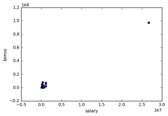
In order to scan for any potential outliers in the dataset, we first look at a scatterplot between the salary and bonus (Shown in the first plot below).
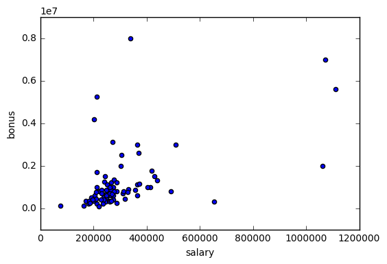
Cleary, there is an outlier in the top-right corner of the plot that requires further examination. This point happens to be the ‘TOTAL’ line in the financial information that sums up the various financial metrics within our dataset. Since this observation does not correspond to an employee, it should be removed from the data. There is another observation in the dataset called ‘THE TRAVEL AGENCY IN THE PARK’ that also should be removed. After removing these 2 observations, we duplicate the plot above and notice that there are no points that are extremely different than the rest (Shown in the second plot below)
### REMOVE OUTLIERS ###

### Create scatterplot of salary and bonus to detect
### any potential outliers

plt.figure(1)
for key, value in data_dict.items():
    salary = data_dict[key]['salary']
    bonus = data_dict[key]['bonus']
    plt.scatter(salary, bonus)
plt.xlabel("salary")
plt.ylabel("bonus")
plt.show()

### The outlier that we see in the above scatterplot is the
### TOTAL line that contains the sum of all the salary and
###  bonus values and needs to be removed
data_dict.pop("TOTAL",0)

### There is another outlier that needs to be removed
data_dict.pop("THE TRAVEL AGENCY IN THE PARK",0)

### Create scatterplot of salary and bonus to ensure all outliers
### have been eliminated

plt.figure(2)
for key, value in data_dict.items():
    salary = data_dict[key]['salary']
    bonus = data_dict[key]['bonus']
    plt.scatter(salary, bonus)
plt.xlabel("salary")
plt.ylabel("bonus")
plt.show()
Create New Feature
In an attempt to increase the accuracy of the algorithm to identify the POIs in the dataset, a new feature was created. This feature is the ratio between the bonus and the salary of each employee. The rationale behind this is that if an employee has an unusually large bonus to salary ratio, they must rely a lot more on their bonus than their salary for a higher income and would therefore be more inclined to engage in illegal or unethical behavior to boost company performance, which would then in turn lead to a higher bonus.
### CREATE NEW FEATURE
for key, value in data_dict.items():
    if (data_dict[key]['bonus']) != 'NaN' and \
    (data_dict[key]['salary']) != 'NaN':
        data_dict[key]['bonus_salary_ratio'] = \
        (float(data_dict[key]['bonus'])/float(data_dict[key]['salary']))
    else:
        data_dict[key]['bonus_salary_ratio'] = 'NaN'

### Store to my_dataset for easy export below.
my_dataset = data_dict

### Extract features and labels from dataset for local testing
data = featureFormat(my_dataset, features_list, sort_keys = True)
labels, features = targetFeatureSplit(data)
Feature Selection
The features used in the algorithm were determined using the SelectKBest method.
It was determined that K = 5 and K = 6 have the highest accuracy, precision and recall scores. In order to avoid over fitting the model, it is better to go with the model with less features given equal performance. The output below outlines which features were selected for the final algorithm along with their scores.
### Select K best features
k = 5
skb = SelectKBest(k = k)

### Feature Importance
skb.fit(features, labels)
scores = -np.log10(skb.pvalues_)
scores /= scores.max()
indices = np.argsort(scores)[::-1]
for i in range(5):
    print("feature no. {}: {} ({})".format(i+1,features_list[indices[i]+1],scores[indices[i]]))
updated_features_list = list(features_list[i+1] for i in indices[0:k])

updated_features_list.insert(0,'poi')
print('Updated features list: ', updated_features_list)
feature no. 1: exercised_stock_options (1.0)
feature no. 2: total_stock_value (0.978860444846489)
feature no. 3: bonus (0.863725845607769)
feature no. 4: salary (0.7767175626081195)
feature no. 5: deferred_income (0.528756607360408)
Updated features list:  ['poi', 'exercised_stock_options', 'total_stock_value', 'bonus', 'salary', 'deferred_income']
Feature Scaling
The algorithm was tested by applying a Min-Max Scaler. It turns out that the accuracy, precision and recall scores remain the same with the deployment of feature scaling. This means that featuring scaling did not add to better performance of our model. Since the purpose of feature scaling is to normalize the feature values, it turns out in our case that the large range of the values plays a crucial role in separating the POIs from the non-POIs. Therefore, feature scaling was not used in the final algorithm.
### FEATURE SCALING

### Initialize Standard and Min-Max Scaler
Standard_scaler = StandardScaler()
Min_Max_scaler = MinMaxScaler()
Algorithm Selection and Paramter Tuning
The algorithm that I ended up using to classify POIs and non-POIs was the Gaussian Naïve Bayes algorithm. The other algorithm that I tried was the Decision Tree Classifier.
Tuning the parameters of an algorithm simply means going through the process of optimizing the parameters of your algorithm that provides the best performance. In our case, this means selecting the parameters of our algorithm that maximize the accuracy, precision or recall scores in the classification of POIs and non-POIs. If the parameters are not tuned correctly, the algorithm will not perform optimally and thus have a higher likelihood of misclassifying the labels correctly. I used parameter tuning for the Decision Tree Classifier in order to ensure the most accurate model was utilized.
### ALGORITHM SELECTION

### Naive Bayes
#clf = Pipeline(steps=[("scaling", Min_Max_scaler),("NaiveBayes",GaussianNB())])
clf = Pipeline(steps=[("NaiveBayes",GaussianNB())])

### Decision Tree
# tree = tree.DecisionTreeClassifier()
# parameters = {'tree__criterion': ('gini','entropy'),
#               'tree__splitter':('best','random'),
#               'tree__min_samples_split':[2, 10, 20],
#                 'tree__max_depth':[10,15,20,25,30],
#                 'tree__max_leaf_nodes':[5,10,30]}
# #pipeline = Pipeline(steps=[('scaler', Min_Max_scaler), ('pca',PCA(n_components = 2)), ('tree', tree)])
# pipeline = Pipeline(steps=[('scaler', Min_Max_scaler), ('tree', tree)])
# #pipeline = Pipeline(steps=[('tree', tree)])

# cv = StratifiedShuffleSplit(labels, 100, random_state = 42)
# gs = GridSearchCV(pipeline, parameters, cv=cv, scoring='accuracy')
# gs.fit(features, labels)
# clf = gs.best_estimator_
Validation and Evaluation
Validation is the process in which we use a subset of our training data to tune the parameters of the algorithm. If this step is done incorrectly, you run the risk of over fitting your model that will perform very good on the training set but will do very poorly on the test set. For my algorithm, I used the StratifiedShuffleSplit function to split the data into training and tests for validation purposes.
I evaluated by algorithm based on the precision and recall scores. For my algorithm, I was able to achieve an accuracy, precision and recall scores of 0.85, 0.49 and 0.38, respectively. Precision refers to the probability that an employee identified as a POI is actually a POI and recall refers to the probability of my algorithm in positively identifying a POI.
### VALIDATION AND EVALUATION

test_classifier(clf, my_dataset, updated_features_list)
Pipeline(steps=[('NaiveBayes', GaussianNB(priors=None))])
    Accuracy: 0.85464   Precision: 0.48876  Recall: 0.38050 F1: 0.42789 F2: 0.39814
    Total predictions: 14000    True positives:  761    False positives:  796   False negatives: 1239   True negatives: 11204