The Baseball Data was used to answer the following questions:
Are salaries higher in 2015 than in 1985?
Does the mean salary increase with the year?
Do a player salaries have a higher correlation with total runs or homeruns?
# Import packages
import csv
import numpy as np
import pandas as pd
import pylab as P
import matplotlib.pyplot as plt
%matplotlib inline

# Use pandas csv reader to read in the salary data
salary_df = pd.read_csv("Data/Salaries.csv", header = 0)

# Question: Are salaries higher in 2015 than in 1985?

# Compare salary statistics between 1985 and 2015
salaryData_1985 = salary_df[salary_df['yearID'] == 1985]['salary']
salaryData_2015 = salary_df[salary_df['yearID'] == 2015]['salary']

print('The median salary in 1985 is $%.2f' % np.median(salaryData_1985))
print('The median salary in 2015 is $%.2f' % np.median(salaryData_2015))

print('The mean salary in 1985 is $%.2f' % np.mean(salaryData_1985))
print('The mean salary in 2015 is $%.2f' % np.mean(salaryData_2015))

print('The max salary in 1985 is $%.2f' % np.amax(salaryData_1985))
print('The max salary in 2015 is $%.2f' % np.amax(salaryData_2015))

# Look at the distribution of the salary data
# Plot histrograms of 1985 and 2015 salaries
plt.figure(1)
plt.subplot(211)
plt.title('Histogram of Salary data in 1985 and 2015')
plt.hist(salaryData_1985)
plt.xlabel('Salary')
plt.ylabel('Frequency - 1985')

plt.subplot(212)
plt.hist(salaryData_1985)
plt.xlabel('Salary')
plt.ylabel('Frequency - 2015')

plt.show()
The median salary in 1985 is $400000.00
The median salary in 2015 is $1880000.00
The mean salary in 1985 is $476299.45
The mean salary in 2015 is $4301276.09
The max salary in 1985 is $2130300.00
The max salary in 2015 is $32571000.00
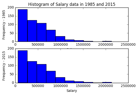
The salaries are tentatively higher in 2015 than in 1985.
The histograms were plotted to see the distibution of our salaries. The fact that the distribution is not normal, but instead right skewed, gives us an idea of the type of model we can use if we wanted to develop a predictive model to determine the salaries.
# Question: Does the mean salary increase with the year?

# Get all the unique years in the dataset
years = np.unique(salary_df['yearID'])

# Initialize empty list to store mean salaries
mean_salary = []

# Get average salary for each year
for each_year in years:
    year_salaries = salary_df[salary_df['yearID'] == each_year]['salary']
    mean_salary.append(np.mean(year_salaries))

# Convert mean salaries list to numpy array
mean_salary = np.array(mean_salary)

# Plot the year vs. mean salary line plot
plt.plot(years, mean_salary)
plt.xlabel('Year')
plt.ylabel('Mean Salary ($)')
plt.show()
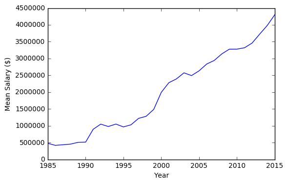
The long term trend shows that the mean salary tends to increase over time.
A line graph was plotted so that we can see the relationship between year and the mean salary. Although the relationship between year and mean salary is not perfectly linear, we can still get away by using a basic linear model if we wanted to develop a predictive model. One can also argue that the curve is non-linear and we may have to go beyond the basic linear model if we were to develop a predictive model.
# Question: Do a player salaries have a higher correlation with total runs or homeruns?

# Define function to calculate correlations
def correlations(DF, VarA, VarB):
    #Inputs: Dataframe, Variable A and Variable B
    return DF[VarA].corr(DF[VarB])

# Use pandas csv reader to read in the batting and salary data
batting_df = pd.read_csv("Data/Batting.csv", header = 0)
salary_df = pd.read_csv("Data/Salaries.csv", header = 0)

# Look at the unique years in which the data for
# runs and homeruns is missing
missing_runs = batting_df[batting_df['R'].isnull()][['yearID']]
unique_missing_runs_years = np.unique(missing_runs['yearID'])
print('There are missing values for runs in years %.0f - %.0f' % \
      (unique_missing_runs_years[0], unique_missing_runs_years[-1]))

missing_homeruns = batting_df[batting_df['HR'].isnull()][['yearID']]
unique_missing_homeruns_years = np.unique(missing_homeruns['yearID'])
print('There are missing values for homeruns in years %.0f - %.0f' % \
      (unique_missing_homeruns_years[0], unique_missing_homeruns_years[-1]))

# Data Cleaning

# Create a new column duplicating the runs and homeruns columns and
# replacing missing runs and homeruns data with 0s
batting_df['Runs'] = batting_df['R']
batting_df.loc[batting_df['Runs'].isnull()] = 0

batting_df['HomeRuns'] = batting_df['HR']
batting_df.loc[batting_df['HomeRuns'].isnull()] = 0

# Data Analysis

# Merge the batting and salary dataframes
dfMerged = pd.merge(batting_df, salary_df, on = ['yearID', 'playerID'], how = 'inner')

# Calculate correlations between Runs / Homeruns and Salary
Runs_Salary_Corr = correlations(dfMerged, 'Runs', 'salary')
HomeRuns_Salary_Corr = correlations(dfMerged, 'HomeRuns', 'salary')

# Results

# Print out the results
print('\nThe correlation between a player\'s total runs and salary is %.2f ' % Runs_Salary_Corr)
print('The correlation between a player\'s homeruns and salary is %.2f ' % HomeRuns_Salary_Corr)
There are missing values for runs in years 1973 - 1999
There are missing values for homeruns in years 1973 - 1999

The correlation between a player's total runs and salary is 0.22
The correlation between a player's homeruns and salary is 0.27
Player salaries have a higher correlation with homeruns than total runs.
Limitations: The missing missing values for total runs and homeruns was replaced with zeros. This method may not reflect reality. Other ways to deal with missing missing data for total runs and homeruns could be:
1. Replace the missing values with mean values instead of zeros
2. Completely remove all items where there are any missing values
3. Interpolate the values
Further steps include adding confidence intervals when caclulating average salary values so that we can be aware of the uncertainty in our calculations.
The correlations were calculated to get an idea of whether the total runs or homeruns would be good features to include in a model if we were to develop a predictive model. The limitation of doing correlations on single variables like we did above is that the combined impact of multiple variables is not considered.